This tutorial will show you how to generate a hill-shaded topographic map using data downloaded from the National Map Viewer. We will be plotting an regional map of the Laramie Range using 1/3 Arc Second (~10 m) data. I went onto National Map and selected the area of interest and then downloaded the data with the format “IMG”. I am pretty sure this script will work with any data format. You can download the zip file containing my script and the data here.
1) Convert the .img file from the National Map Viewer into a netCDF grid that can be plotted by GMT:
gdal_translate -b 1 -of GMT ${path2ElevFile}imgn42w106_13.img LR-ElevationLatLong.grd
This command extracts the elevations from the .img file. The “-b” flag represent the first (and only) band, which represents the elevations. I am setting output format to GMT using the “-of” flag. Finally, since this is in a c-shell I can use variables. I set the path to the downloaded .img file using a variable. I then called the output GMT (netCDF) grid file as LR-ElevationLatLong.grd. Now that we have the elevations in the correct format it is easy sailing.
2) I like to cut the grid file to my particular area of interest. I elected to set "-R-105.4700/-105.3085/41.17/41.3000”, which is a subset of the region. I do this to create smaller files, so that the PDF or PostScript file are not huge. To do this use the grdcut command
gmt grdcut LR-ElevationLatLong.grd -GBW-grdFile.grd $region
Where LR-ElevationLatLong.grd is the file we just created and the output file is specified using the “-G” flag. Finally $region is the variable that sets the “-R” flag.
3) Build the hill-shade, or gradient file, to overlay on the DEM. This command essentially illuminates the grid file. You can control the azimuth and angle of the sun. This is the file that makes the DEM look like topography because it amplifies the small changes in elevation.
set misc = "-A90/50 -fg"
gmt grdgradient LR-ElevationLatLong.grd -GLR_topo.grad $misc
The “-A” flag controls the illumination. The first number is the azimuth and the second number is the angle. In this case the sun is directly north and 50 degrees from the horizon. You can see this in the shadows. The “-fg” flag tells GMT to convert the latitude and longitude to an x-y grid so that it can apply the fill. Finally specify elevation and the output file using the “-G” flag. I tend to put a .grad extension on these types of files, but you can call it whatever you want.
4) Build a color pallet to fill the elevations
set misc = "-Chaxby -D -V -T2400/2700/10”
gmt makecpt $misc >! LR_topo.cpt
I typically use makecpt instead of grd2cpt because I can control the minimum and maximum elevations and the contour interval. The “-C” flag controls the color pallet, the “-D” flag fills in values above and below the maximum values, and the “-T” flag allows you to set the color intervals. In this case the “-T” flag saying fill from 2400 to 2700 m in intervals of 10 meters.
6) Plot the image using grdimage or grdview
gmt grdimage LR-ElevationLatLong.grd $region $projection -ILR_topo.grad -CLR_topo.cpt $open -Y2i >! $psFile
I tend to always us gdrimage because that’s how I learned. Another alternative, with almost exactly the same input parameters, is grdview. In order to plot the hill-shade you have to specify the gradient file generated using grdgradient with the “-I” flag. You also specify the color pallet file you generated using makecpt using the “-C” flag.
7) Plot the scale bar
gmt pscoast -W $region $projection -Lf-105.34/41.16/41.20/5.0k+u--LABEL_FONTSIZE=10 $add >> $psFile
A lot of times on regional maps it is nice to have a scale bar. In this case you use the psbasemap command. The -Lf flag controls the location of the scale bar.
8) Plot the color bar
gmt gmtset FONT_LABEL 14p
gmt gmtset MAP_LABEL_OFFSET -0.50i
gmt psscale -D2i/-0.5i/2i/0.25ih -CLR_topo.cpt $add -B100:"Elevation (m)":wSen >> $psFile
gmt gmtset FONT_LABEL 16p
gmt gmtset MAP_LABEL_OFFSET 0.3c
This is one of my favorite tricks. There is probably a more elegant way to do it, but this works for me. To place the text inside (instead of below) the color bar you set the default parameters before calling the command. The MAP_LABEL_OFFSET will shift the text up and the FONT_LABEL controls the size of the text. Don’t forget to reset the default parameters after you plot the color bar! If you don’t the rest of the axes in your plots will be messed up.
9) Plot inset (optional)
set subregion = "-R-117.5/-100/36.8/49"
set subprojection = "-JM2.45i"
gmt psbasemap $subregion $subprojection -B100/100:."":wsen $add -X4.15i -Y4.75i >> $psFile
set misc = "-Ggray -Sblue -Na/1p"
gmt pscoast $subregion $subprojection $misc $add >> $psFile
set misc = "-Sa0.3i -W0.1p -G255/255/0 -:"
gmt psxy $subregion $subprojection $add $misc << EOF >> $psFile
41.23 -105.41
EOF
set misc = "-Sc0.1i -W0.1p -G255/0/0 -:"
gmt psxy $subregion $subprojection $close $misc << EOF >> $psFile
39.687 -104.706
EOF
For talks and posters it’s always nice to have a good inset map. This is my standard configuration. You essentially select a subregion of interest. In my case I typically go from the Idaho-Montana border t0 just East of Colorado border. You then move the inset around using the “-X" and "-Y” flags. This can get a little tedious, but once you get the location right it is well worth it.
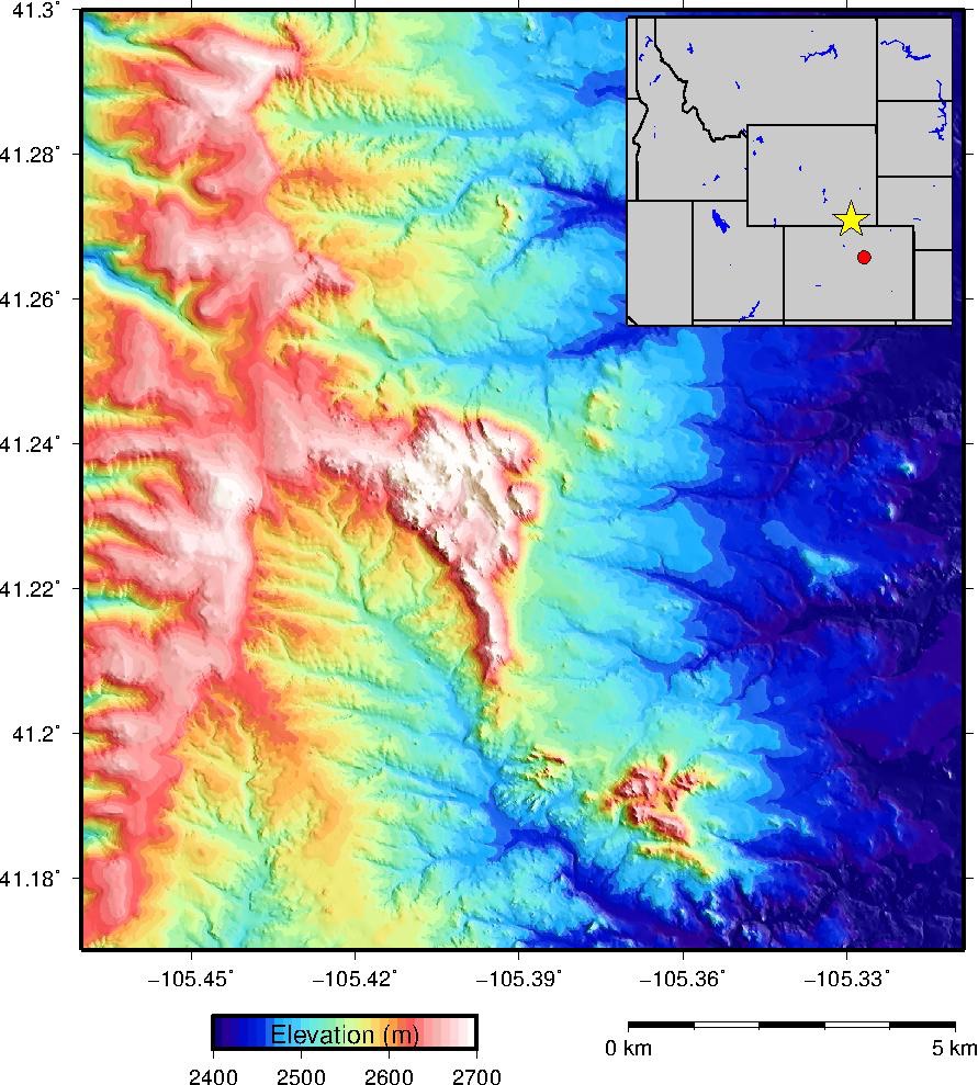
The final map generated from the script above. This is a pretty good boiler script for any hill-shaded topogarphic map. It even works for LiDAR!