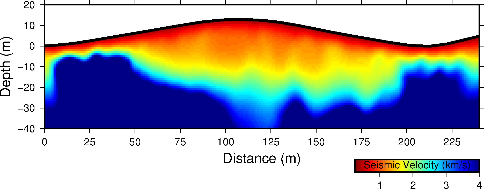
This is one of my most commonly used GMT scripts. I have simplified it quite a bit, because you can add a lot of things to these plots such as a ray path mask, or the rays themselves. By the end of this quick tutorial you should be able to generate the plot shown on the right. I have provided the data, topography, and topography fill in a zip file that you can download here.
Setting the Basic Parameters
The first part of the script I use to set all of my variables. The region, or -R, will control the interpolation area selected. The seismic refraction data that I have provided in the .zip file contains velocities from 0 to 237.5 m and has a maximum height of about 15 m and goes to a depth ~35 m. Thus an appropriate selection of the region is shown below:
set region = "-R0/240/-40/20”
The Projection variable controls the size, and thus the vertical exaggeration of the plot area. I tend to like this aspect ratio, but you can play around with the sizes as you please. The i appended to the end of the numbers represents inches. So the interpolated area will be 7 inches long and 2 inches high.
set projection = "-JX7i/2i”
These are just settings to make sure the commands are either opening, appending or adding the postscript file.
set open = "-K -V"
set add = "-O -K -V"
set close = "-O -V”
This set of commands controls the name of the final plotted file. Keep in mind; if you don’t have the command ps2pdf (not GMT related) installed, then the pdf file name is unnecessary.
set psFile = "geophysicalTransect.ps"
set pdfFile = “geophysicalTransect.pdf"
This is a flag that I am using to control if contours show up on the plot. If it is valued an anything other than 1 then contours will be absent. To add contours to the plot set this value to 1.
set contourPlot = 0
Do the Interpolation
GMT contains a few methods for interpolating data. My personal favorite is the surface command. There is an entire paper written on this subject but essentially this method is ideal for geophysical data because it holds the second derivative continuous (Smith and Wessel, 1990; reference linked at the bottom of page). The interpolation in this script happens over the the following five lines of code.
These are variables used to set the dx and dy (or dz) of the final interpolated grid. You can set the units, but if you leave them blank it will use whatever units are in the file.
set dx = 1
set dy = 1
The seisFile variable is the variable with the location of the text file containing the seismic velocity section. This file is a list of x, y, and z pairs in any order. You can scatter plot these with psxy if you really want to.
set seisFile = xyzFile.temp
This command decimates the data to the prescribed dx and dy with the -I flag. This is important because if you have data points that are smaller than your grid spacing, you get artifacts that look like oscillations in the interpolation (Smith and Wessel, 1990).
gmt blockmean $seisFile $region -I${dx}/${dy} > tmpSeis.beam
This command applies the Smith and Wessel (1990) algorithm and generates a netCDF (GMT format) grid file that has even spacing that follow the dx and dy from the -I flag. The output grid file name is controlled using the -G flag. If you want an extremely smooth looking plot with no interpolation artifacts you can set the -I flag larger in the blockmean command and make the -I numbers smaller for the surface command. If you make the uniform grid smaller (-I flag of the surface command) the image will appear very smooth. I like to plot geophysical transects, seismic velocities in particular, with very smooth parameters because we do not expect to see large contrasts in seismic velocities from the inversion.
gmt surface tmpSeis.beam -GseisGrid.grd -I${dx}/${dy} $region
Next we need to generate the color pallet that will be used to plot the image. The -T flag is what controls the boundaries of the color scale. The first value assigns the value to the low end of the selected color palette and the last number is essentially the contour interval for the colors to change. This command will have 75 ([4-0.25]/0.05 = 75) equally spaced colors. For this plot I want my minimum value to be 0.25 (these are in km/s) and the highest value to be 4. With a color palette of jet (-CJet) this means that 0.25 will be blue and 4 will be red. The -I flag inverts the colors assigning 0.25 to red and 4 to blue. The final flag, -D means that if there is value less than 0.25 or greater than 4 they will be filled in with the end member colors. In other words if it comes across a velocity of 5.0 km/s it will plot as the same color as something with 4 km/s.
gmt makecpt -T0.25/4/0.05 -D -I -CJet > seismicVels.cpt
This command plots the interpolated grid with the created color palette (-CcolorPaletteName.cpt). This also is the first time we are actually writing to the postscript file, that is why we add the $open variable. We also shift this grid straight up 5 inches (-Y5i). If you look at the postscript file at this point you will see that surface interpolated the entire rectangle. We need to lift off, or hide, the area above the topography.
gmt grdimage seisGrid.grd $region $projection -CseismicVels.cpt -Y5i $open >! $psFile
If you set the contour variable to true then you will plot thick contours over the seismic data. This must be done prior to lifting, or hiding, the topography. The -A flag controls the contour label interval, in this case 1 km/s. The -W flag controls the thickness of the contour lines. The tmpSeis.beam is the data file that was decimated by the blockmean.
if $contourPlot == 1 then
gmt pscontour tmpSeis.beam -A1 -W2.5p $region $projection $add >> $psFile
endif
Now we just need to white out the area above the topography. To do this I have provided you with the topographic file (topoFile.temp) and a fill file (topoFile_fill.temp). The fill file is identical to the topographic profile with the exception that I added five points at the end of the file to complete a polygon. I usually use large numbers to make sure the polygon completes why outside of the desired region. In these lines I white out the area and then plot a thick black line. See my tutorial on plotting an x-y plot for more information on the psxy command.
set misc = "-G255/255/255"
gmt psxy topoFile_fill.temp $region $projection $misc $add >> $psFile
set misc = "-W3p"
gmt psxy topoFile.temp $region $projection $misc $add >> $psFile
Next we plot the proper labels around the interpolated image. Once again for more information on the psbasemap command see my tutorial on plotting an x-y plot.
gmt psbasemap $region $projection -B25:"Distance (m)":/10:"Depth (m)":WSen $add >> $psFile
Finally we need to plot the color bar and close the file. I don’t do this in the smoothest way, but it does work well. I use the GMT defaults to move the text label of the color bar into the color bar itself. I change the font size to smaller using FONT_LABEL and move it inside the color bar used MAP_LABEL_OFFSET. The -D flag controls the size and location of the color bar. The first number is the x distance from the original zero point or plotting location. The second number is the y distance from the original zero point or plotting location. The third number is the length/height of the color bar. the final number is the width of the color bar. The -C flag is the color palette used to plot the data. I then set the defaults back to what they were prior to adjusting them. I use the close flag to signify this is the last command going into the postscript file.
gmt gmtset FONT_LABEL 12p
gmt gmtset MAP_LABEL_OFFSET -0.5i
gmt psscale -D6i/-0.5i/2.0i/0.2ih -CseismicVels.cpt $close -B1:"Seismic Velocity (km/s)":wSen >> $psFile
gmt gmtset MAP_LABEL_OFFSET 0.3c
gmt gmtset FONT_LABEL 16p
This command converts the postscript file into a jpeg with a resolution of 240 dpi (fairly high quality). It also clips off any extra white space, leaving you with the image in the upper right hand corner of this page.
Cited Reference
Smith, W., and P. Wessel (1990), Gridding with continuous curvature splines in tension, GEOPHYSICS, 55(3), 293–305, doi:10.1190/1.1442837.