I took this class because so much of geophysics involves running inversions. Since the majority of the math I do is in Matlab I wanted to learn how differential equations are solved numerically. This course focused on solving differential equations using finite difference approximation. We went through the derivation of the finite difference approximation, learned how to use Runge-Kutta methods, and steepest decent methods to solve different kinds of boundary value problems (BVP). Since these are numerical solutions, everything is dependent on the boundary conditions. What I found is that the accuracy of the numerical methods depend on on the mesh or grid sized used to estimate the solution. Some methods are better than others when using larger mesh sizes. I think this was an important concept to pull away from this course because in geophysics most, if not all, of the forward models used are based on numerical approximation. It is important to make sure the mesh size of the forward modeling code is small enough so that you trust the solutions.
Solving Non-linear Differential Equations
OOne of the most powerful attributes of using numerical differential equations is that it allows you to estimate solutions to non-linear equations that can’t be solved analytically. For example we used Newton’s method to solve the following non-linear equation for the provided boundary conditions. This equation represents how the angle of a string changes as a weight swings back and forth (i.e. pendulum problem). The problem is non-linear because the second derivative of the angle is dependent on the the angle itself. Below is the equation with two sets of boundary conditions that were solved:
Newton’s method is used to find where a function passes through through another function, say y = 0. The animation below (http://en.wikipedia.org/wiki/Newton's_method) illustrates the concept:
So for the non-linear problem I used Newtons method to estimate the homogeneous equation. I used a first order approximation for the second derivative:
Once the homogeneous equation above has been solved, I have a guess at all of the values of theta. These guesses can be substituted in on the right hand side of the non-linear equation. After the substation I can solve the non-linear system:
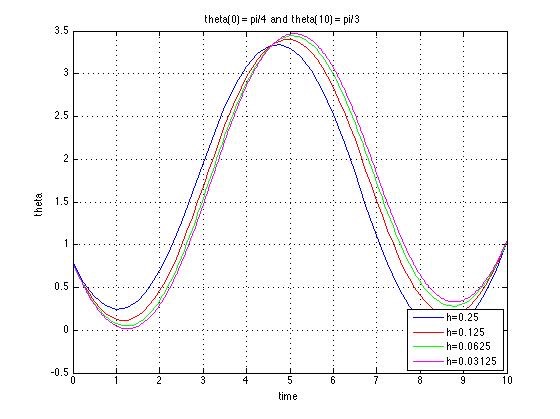
The graphical results of the non-linear equation for the second set of boundary conditions and various step sizes (i.e. mesh sizes) is shown below:
Solving the Laplace Equation
We worked with Laplace equation a lot during the semester. I am glad we did, because this equation comes up a lot in geophysical modeling. For example, if you assume an isotropic hydraulic conductivity and steady state flow (i.e. no storage), the groundwater flow equation that I learned in geohydrology reduces to the same form. Below I give an example that we solved in this class. The top equation is the Laplace equation. It was solved it numerically with the boundary conditions provided below.
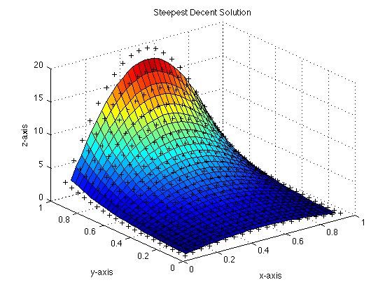
The graphical solution is shown below. I solved this equation using my own steepest-decent algorithm. The small plus signs represent the numerical grid at which the solution was estimated.
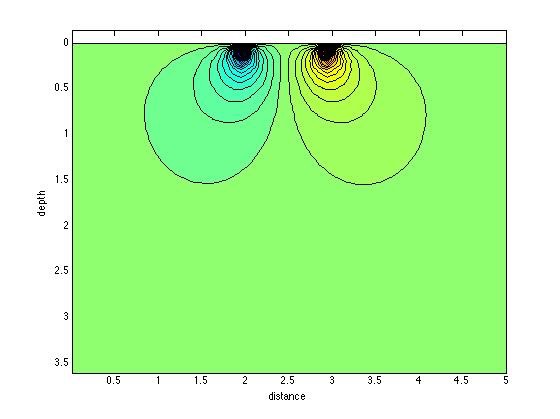
I adapted this code so that I could write my own resistivity forward modeling code. Although the boundary conditions are not physically representative of the resistivity system, I did succeed in calculating the voltage response for an input current at two locations. Below I have contoured the voltage lines. Conceptually, the current would flow perpendicular to these contour lines. The case below is calculated for a homogeneous conductive earth (~1 S/m). Although my code is very basic and computationally expensive, I understand how the forward modeling codes, such as Earth Imager© works.